Great new way to handle Missing Values
Missing values in datasets are a common challenge in data analysis and can significantly impact the quality of research or predictive models. They arise due to various reasons, such as errors in data collection, non-response in surveys, or disruptions in data transmission. The handling of these missing values is crucial, as improper treatment can lead to biased results and incorrect conclusions.
There are several strategies for dealing with missing data, each with its advantages and limitations. They can be listed as follows: Deletion, Imputation, Synthetization. The approach we take to handle the missing data, very much depends on the nature of the missing data. There are three main types of missing data, each with different implications:
Missing Completely at Random (MCAR):
- When the probability of a value being missing is the same for all cases, the data is said to be missing completely at random.
- In MCAR, the missingness of data is unrelated to any of the study variables or to the missing data itself.
- If data are MCAR, most handling methods, including simple ones like deletion or mean imputation, are unlikely to introduce bias.
Missing at Random (MAR):
- Data is missing at random if the missingness is related to some observed data and not to the value of missing data itself.
- For instance, if younger participants are more likely to skip a survey question, the missingness is related to the ‘age’ variable but not necessarily to the missing question’s answers.
- Handling MAR often requires more sophisticated methods, such as multiple imputation, which can model the missingness based on observed data.
Missing Not at Random (MNAR):
- Data is missing not at random if the missingness is related to the value of the missing data itself.
- For example, individuals with lower income might be more likely to skip income-related questions.
- MNAR is the most challenging type of missing data to handle because it requires understanding the mechanism behind the missingness and often needs complex statistical methods or domain expertise for appropriate handling.
In cases where the missing data points are MCAR and missing values don’t make a large part of the dataset, we could simply delete the observations (rows) which have missing values without loosing relevant information from the dataset.
If the missing values are MAR, and/or the missing values make a large part of the dataset, Imputation is a good way to proceed. There are various ways of performing Imputation:
- Mean/Median/Mode Imputation: Replace missing values with the mean, median, or mode of the column.
- K-Nearest Neighbors (KNN) Imputation: Replace a missing value using the KNN algorithm, which finds the nearest neighbors according to a given distance measure.
- Regression Imputation: Use regression models to estimate and replace missing values
Finally, in case the data is MNAR and especially if the missing values are plentiful, there is no clear way of action. In such cases missing datapoint can be either imputed, synthesized or otherwise generated through a number of other techniques which are often tailored depending on the end goal of the data analysis.
While both imputation and synthesizing data address the issue of incomplete data, imputation focuses on filling in gaps in an existing dataset, adhering closely to its original structure. In contrast, data synthesis involves creating new data points, often for broader purposes like data augmentation, privacy preservation, or when actual data is unavailable. Synthesizing data includes methods like data simulation, where a model is built to generate data points that mimic the distributions of real data. Techniques like bootstrapping or generative models (e.g. Generative Adversarial Networks) are often used.
The approach I wish to introduce is referred to as the “Hard-Impute” and it was first published by Mazumder, Hastie, and Tibshirani. It is an Imputation technique, best suited for MAR and MCAR scenarios.
The Hard-Impute
Imputation methods aim at addressing missing values by identifying the patterns and relationships within the available, non-missing data. These identified structures are then utilized to estimate and replace the missing values effectively. An example of a very popular imputation method is the K-Nearest Neighbors Imputation, however it suffers from the same weakness as the KNN clasifier, which is its high sensitivity to irrelevant features.
The Hard-Impute utilizes the correlation structure behind the features of the dataset in order to proxy for the missing values. It does so by iteratively calculating the principal components of the dataset, and using the PCA scores and vector loadings to reconstruct the original values. This might sound like a handful, so let’s dive deeper into that following an example.
Below is a well-known US Arrests dataset from which we have removed 20 values by random. The dataset showcases the number of arrests per 100,000 residents for crimes such as assault, murder, and gender crimes in each of the 50 US states in 1973. The dataset is available here
US Arrests Data
| # | State | Murder | Assault | UrbanPop | GendCrimes |
|---|---|---|---|---|---|
| 1 | Alabama | 13.2 | 236.0 | 58.0 | 21.2 |
| 2 | Alaska | 10.0 | 263.0 | 48.0 | 44.5 |
| 3 | Arizona | 8.1 | 294.0 | 80.0 | 31.0 |
| 4 | Arkansas | 8.8 | 190.0 | 50.0 | NaN |
| 5 | California | 9.0 | 276.0 | 91.0 | 40.6 |
| 6 | Colorado | 7.9 | 204.0 | 78.0 | 38.7 |
| 7 | Connecticut | 3.3 | 110.0 | 77.0 | 11.1 |
| 8 | Delaware | 5.9 | 238.0 | 72.0 | 15.8 |
| 9 | Florida | 15.4 | 335.0 | 80.0 | 31.9 |
| 10 | Georgia | NaN | 211.0 | 60.0 | 25.8 |
| 11 | Hawaii | 5.3 | 46.0 | 83.0 | 20.2 |
| 12 | Idaho | 2.6 | 120.0 | 54.0 | 14.2 |
| 13 | Illinois | 10.4 | 249.0 | 83.0 | 24.0 |
| 14 | Indiana | 7.2 | 113.0 | 65.0 | 21.0 |
| 15 | Iowa | 2.2 | 56.0 | 57.0 | NaN |
| 16 | Kansas | 6.0 | 115.0 | 66.0 | 18.0 |
| 17 | Kentucky | 9.7 | NaN | 52.0 | 16.3 |
| 18 | Louisiana | 15.4 | 249.0 | 66.0 | 22.2 |
| 19 | Maine | 2.1 | 83.0 | 51.0 | 7.8 |
| 20 | Maryland | 11.3 | 300.0 | 67.0 | 27.8 |
| 21 | Massachusetts | 4.4 | NaN | 85.0 | 16.3 |
| 22 | Michigan | 12.1 | 255.0 | 74.0 | 35.1 |
| 23 | Minnesota | NaN | 72.0 | 66.0 | 14.9 |
| 24 | Mississippi | 16.1 | 259.0 | 44.0 | 17.1 |
| 25 | Missouri | 9.0 | 178.0 | 70.0 | 28.2 |
| 26 | Montana | 6.0 | NaN | 53.0 | 16.4 |
| 27 | Nebraska | 4.3 | NaN | 62.0 | 16.5 |
| 28 | Nevada | 12.2 | 252.0 | 81.0 | 46.0 |
| 29 | New Hampshire | 2.1 | 57.0 | 56.0 | 9.5 |
| 30 | New Jersey | 7.4 | 159.0 | 89.0 | 18.8 |
| 31 | New Mexico | NaN | 285.0 | 70.0 | 32.1 |
| 32 | New York | 11.1 | 254.0 | 86.0 | 26.1 |
| 33 | North Carolina | 13.0 | 337.0 | 45.0 | 16.1 |
| 34 | North Dakota | 0.8 | NaN | 44.0 | 7.3 |
| 35 | Ohio | 7.3 | 120.0 | 75.0 | 21.4 |
| 36 | Oklahoma | 6.6 | 151.0 | 68.0 | NaN |
| 37 | Oregon | NaN | 159.0 | 67.0 | 29.3 |
| 38 | Pennsylvania | 6.3 | 106.0 | 72.0 | NaN |
| 39 | Rhode Island | NaN | 174.0 | 87.0 | 8.3 |
| 40 | South Carolina | 14.4 | 279.0 | 48.0 | 22.5 |
| 41 | South Dakota | 3.8 | 86.0 | 45.0 | 12.8 |
| 42 | Tennessee | NaN | 188.0 | 59.0 | 26.9 |
| 43 | Texas | 12.7 | 201.0 | NaN | 25.5 |
| 44 | Utah | 3.2 | NaN | 80.0 | 22.9 |
| 45 | Vermont | NaN | 48.0 | 32.0 | 11.2 |
| 46 | Virginia | 8.5 | 156.0 | 63.0 | 20.7 |
| 47 | Washington | 4.0 | 145.0 | 73.0 | 26.2 |
| 48 | West Virginia | 5.7 | 81.0 | NaN | 9.3 |
| 49 | Wisconsin | 2.6 | 53.0 | 66.0 | 10.8 |
| 50 | Wyoming | 6.8 | 161.0 | NaN | 15.6 |
The 1st step of the Hard-Impute Algorithm is to standardize the dataset with a mean of 0 and standard deviation of 1, and to replace the mising values with their column/feature means.
Standardized US Arrests Data
| # | State | Murder | Assault | UrbanPop | GendCrimes |
|---|---|---|---|---|---|
| 1 | Alabama | 1.34 | 0.68 | -0.56 | -0.05 |
| 2 | Alaska | 0.55 | 1.00 | -1.27 | 2.41 |
| 3 | Arizona | 0.08 | 1.37 | 1.00 | 0.98 |
| 4 | Arkansas | 0.25 | 0.12 | -1.13 | NaN |
| 5 | California | 0.30 | 1.16 | 1.78 | 2.00 |
| 6 | Colorado | 0.03 | 0.29 | 0.86 | 1.80 |
| 7 | Connecticut | -1.10 | -0.84 | 0.79 | -1.11 |
| 8 | Delaware | -0.46 | 0.70 | 0.43 | -0.62 |
| 9 | Florida | 1.88 | 1.86 | 1.00 | 1.08 |
| 10 | Georgia | NaN | 0.38 | -0.42 | 0.44 |
| 11 | Hawaii | -0.61 | -1.60 | 1.21 | -0.15 |
| 12 | Idaho | -1.27 | -0.72 | -0.85 | -0.78 |
| 13 | Illinois | 0.65 | 0.83 | 1.21 | 0.25 |
| 14 | Indiana | -0.14 | -0.80 | -0.06 | -0.07 |
| 15 | Iowa | -1.37 | -1.48 | -0.63 | NaN |
| 16 | Kansas | -0.44 | -0.78 | 0.01 | -0.38 |
| 17 | Kentucky | 0.47 | NaN | -0.99 | -0.56 |
| 18 | Louisiana | 1.88 | 0.83 | 0.01 | 0.06 |
| 19 | Maine | -1.40 | -1.16 | -1.06 | -1.46 |
| 20 | Maryland | 0.87 | 1.44 | 0.08 | 0.65 |
| 21 | Massachusetts | -0.83 | NaN | 1.36 | -0.56 |
| 22 | Michigan | 1.07 | 0.90 | 0.57 | 1.42 |
| 23 | Minnesota | NaN | -1.29 | 0.01 | -0.71 |
| 24 | Mississippi | 2.05 | 0.95 | -1.56 | -0.48 |
| 25 | Missouri | 0.30 | -0.02 | 0.29 | 0.69 |
| 26 | Montana | -0.44 | NaN | -0.92 | -0.55 |
| 27 | Nebraska | -0.85 | NaN | -0.28 | -0.54 |
| 28 | Nevada | 1.09 | 0.87 | 1.07 | 2.56 |
| 29 | New Hampshire | -1.40 | -1.47 | -0.70 | -1.28 |
| 30 | New Jersey | -0.09 | -0.25 | 1.64 | -0.30 |
| 31 | New Mexico | NaN | 1.26 | 0.29 | 1.10 |
| 32 | New York | 0.82 | 0.89 | 1.43 | 0.47 |
| 33 | North Carolina | 1.29 | 1.89 | -1.49 | -0.58 |
| 34 | North Dakota | -1.72 | NaN | -1.56 | -1.51 |
| 35 | Ohio | -0.12 | -0.72 | 0.65 | -0.03 |
| 36 | Oklahoma | -0.29 | -0.34 | 0.15 | NaN |
| 37 | Oregon | NaN | -0.25 | 0.08 | 0.81 |
| 38 | Pennsylvania | -0.36 | -0.88 | 0.43 | NaN |
| 39 | Rhode Island | NaN | -0.07 | 1.50 | -1.41 |
| 40 | South Carolina | 1.63 | 1.19 | -1.27 | 0.09 |
| 41 | South Dakota | -0.98 | -1.12 | -1.49 | -0.93 |
| 42 | Tennessee | NaN | 0.10 | -0.49 | 0.55 |
| 43 | Texas | 1.21 | 0.26 | NaN | 0.41 |
| 44 | Utah | -1.13 | NaN | 1.00 | 0.13 |
| 45 | Vermont | NaN | -1.58 | -2.41 | -1.10 |
| 46 | Virginia | 0.18 | -0.28 | -0.21 | -0.10 |
| 47 | Washington | -0.93 | -0.42 | 0.50 | 0.48 |
| 48 | West Virginia | -0.51 | -1.18 | NaN | -1.30 |
| 49 | Wisconsin | -1.27 | -1.52 | 0.01 | -1.14 |
| 50 | Wyoming | -0.24 | -0.22 | NaN | -0.64 |
Standardization is a necessary step because PCA is significantly influenced by the different units used to measure the features. Standardization ensures that the principal components reflect the underlying structure of the data in a balanced way, rather than being skewed by arbitrary differences in variable scales and units.
Missing values are replaced with column means (which are 0 by design of standardization)
| # | State | Murder | Assault | UrbanPop | GendCrimes |
|---|---|---|---|---|---|
| 1 | Alabama | 1.34 | 0.68 | -0.56 | -0.05 |
| 2 | Alaska | 0.55 | 1.00 | -1.27 | 2.41 |
| 3 | Arizona | 0.08 | 1.37 | 1.00 | 0.98 |
| 4 | Arkansas | 0.25 | 0.12 | -1.13 | 0.00 |
| 5 | California | 0.30 | 1.16 | 1.78 | 2.00 |
| 6 | Colorado | 0.03 | 0.29 | 0.86 | 1.80 |
| 7 | Connecticut | -1.10 | -0.84 | 0.79 | -1.11 |
| 8 | Delaware | -0.46 | 0.70 | 0.43 | -0.62 |
| 9 | Florida | 1.88 | 1.86 | 1.00 | 1.08 |
| 10 | Georgia | 0.00 | 0.38 | -0.42 | 0.44 |
| 11 | Hawaii | -0.61 | -1.60 | 1.21 | -0.15 |
| 12 | Idaho | -1.27 | -0.72 | -0.85 | -0.78 |
| 13 | Illinois | 0.65 | 0.83 | 1.21 | 0.25 |
| 14 | Indiana | -0.14 | -0.80 | -0.06 | -0.07 |
| 15 | Iowa | -1.37 | -1.48 | -0.63 | 0.00 |
| 16 | Kansas | -0.44 | -0.78 | 0.01 | -0.38 |
| 17 | Kentucky | 0.47 | 0.00 | -0.99 | -0.56 |
| 18 | Louisiana | 1.88 | 0.83 | 0.01 | 0.06 |
| 19 | Maine | -1.40 | -1.16 | -1.06 | -1.46 |
| 20 | Maryland | 0.87 | 1.44 | 0.08 | 0.65 |
| 21 | Massachusetts | -0.83 | 0.00 | 1.36 | -0.56 |
| 22 | Michigan | 1.07 | 0.90 | 0.57 | 1.42 |
| 23 | Minnesota | 0.00 | -1.29 | 0.01 | -0.71 |
| 24 | Mississippi | 2.05 | 0.95 | -1.56 | -0.48 |
| 25 | Missouri | 0.30 | -0.02 | 0.29 | 0.69 |
| 26 | Montana | -0.44 | 0.00 | -0.92 | -0.55 |
| 27 | Nebraska | -0.85 | 0.00 | -0.28 | -0.54 |
| 28 | Nevada | 1.09 | 0.87 | 1.07 | 2.56 |
| 29 | New Hampshire | -1.40 | -1.47 | -0.70 | -1.28 |
| 30 | New Jersey | -0.09 | -0.25 | 1.64 | -0.30 |
| 31 | New Mexico | 0.00 | 1.26 | 0.29 | 1.10 |
| 32 | New York | 0.82 | 0.89 | 1.43 | 0.47 |
| 33 | North Carolina | 1.29 | 1.89 | -1.49 | -0.58 |
| 34 | North Dakota | -1.72 | 0.00 | -1.56 | -1.51 |
| 35 | Ohio | -0.12 | -0.72 | 0.65 | -0.03 |
| 36 | Oklahoma | -0.29 | -0.34 | 0.15 | 0.00 |
| 37 | Oregon | 0.00 | -0.25 | 0.08 | 0.81 |
| 38 | Pennsylvania | -0.36 | -0.88 | 0.43 | 0.00 |
| 39 | Rhode Island | 0.00 | -0.07 | 1.50 | -1.41 |
| 40 | South Carolina | 1.63 | 1.19 | -1.27 | 0.09 |
| 41 | South Dakota | -0.98 | -1.12 | -1.49 | -0.93 |
| 42 | Tennessee | 0.00 | 0.10 | -0.49 | 0.55 |
| 43 | Texas | 1.21 | 0.26 | 0.00 | 0.41 |
| 44 | Utah | -1.13 | 0.00 | 1.00 | 0.13 |
| 45 | Vermont | 0.00 | -1.58 | -2.41 | -1.10 |
| 46 | Virginia | 0.18 | -0.28 | -0.21 | -0.10 |
| 47 | Washington | -0.93 | -0.42 | 0.50 | 0.48 |
| 48 | West Virginia | -0.51 | -1.18 | 0.00 | -1.30 |
| 49 | Wisconsin | -1.27 | -1.52 | 0.01 | -1.14 |
| 50 | Wyoming | -0.24 | -0.22 | 0.00 | -0.64 |
In the 2nd step, the PCA is ran against the standardized dataset. I will not go into detail about PCA in this discussion, but I would just remind the reader that the 1st Principal Component of a set of features is a linear combination of those features that results in the maximum variance
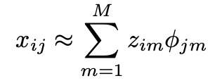
 , where x is our standardized data, p is the number of features, i is the number of observations/rows , z is the first principal component score for each observation i, and fi is the vector loading for each feature p.
PCA algorith outputs i principal component scores and p factor loadings. Due to PCA’s inherent ability to retain maximum information from the dataset, we can represent each data point using the formula:
Naturally, our focus is on approximating the missing values (temporarily replaced with the means of their respective features), while leaving the other data points unchanged.
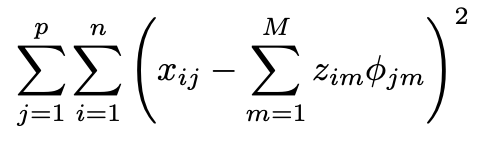
In the 3rd step we would apply the 2nd step iteratively and keep producing the proxies for missing values until the change between the sum of all missing proxy values between 2 iterations falls below a given threshold (in this example it is 0.002)
 < 0.002
Our end result is:
| # | State | Murder | Assault | UrbanPop | GendCrimes |
|---|---|---|---|---|---|
| 1 | Alabama | 1.34 | 0.68 | -0.56 | -0.05 |
| 2 | Alaska | 0.55 | 1.00 | -1.27 | 2.41 |
| 3 | Arizona | 0.08 | 1.37 | 1.00 | 0.98 |
| 4 | Arkansas | 0.25 | 0.12 | -1.13 | -0.01 |
| 5 | California | 0.30 | 1.16 | 1.78 | 2.00 |
| 6 | Colorado | 0.03 | 0.29 | 0.86 | 1.80 |
| 7 | Connecticut | -1.10 | -0.84 | 0.79 | -1.11 |
| 8 | Delaware | -0.46 | 0.70 | 0.43 | -0.62 |
| 9 | Florida | 1.88 | 1.86 | 1.00 | 1.08 |
| 10 | Georgia | 0.33 | 0.38 | -0.42 | 0.44 |
| 11 | Hawaii | -0.61 | -1.60 | 1.21 | -0.15 |
| 12 | Idaho | -1.27 | -0.72 | -0.85 | -0.78 |
| 13 | Illinois | 0.65 | 0.83 | 1.21 | 0.25 |
| 14 | Indiana | -0.14 | -0.80 | -0.06 | -0.07 |
| 15 | Iowa | -1.37 | -1.48 | -0.63 | -1.28 |
| 16 | Kansas | -0.44 | -0.78 | 0.01 | -0.38 |
| 17 | Kentucky | 0.47 | -0.20 | -0.99 | -0.56 |
| 18 | Louisiana | 1.88 | 0.83 | 0.01 | 0.06 |
| 19 | Maine | -1.40 | -1.16 | -1.06 | -1.46 |
| 20 | Maryland | 0.87 | 1.44 | 0.08 | 0.65 |
| 21 | Massachusetts | -0.83 | -0.29 | 1.36 | -0.56 |
| 22 | Michigan | 1.07 | 0.90 | 0.57 | 1.42 |
| 23 | Minnesota | -0.84 | -1.29 | 0.01 | -0.71 |
| 24 | Mississippi | 2.05 | 0.95 | -1.56 | -0.48 |
| 25 | Missouri | 0.30 | -0.02 | 0.29 | 0.69 |
| 26 | Montana | -0.44 | -0.63 | -0.92 | -0.55 |
| 27 | Nebraska | -0.85 | -0.68 | -0.28 | -0.54 |
| 28 | Nevada | 1.09 | 0.87 | 1.07 | 2.56 |
| 29 | New Hampshire | -1.40 | -1.47 | -0.70 | -1.28 |
| 30 | New Jersey | -0.09 | -0.25 | 1.64 | -0.30 |
| 31 | New Mexico | 1.17 | 1.26 | 0.29 | 1.10 |
| 32 | New York | 0.82 | 0.89 | 1.43 | 0.47 |
| 33 | North Carolina | 1.29 | 1.89 | -1.49 | -0.58 |
| 34 | North Dakota | -1.72 | -1.86 | -1.56 | -1.51 |
| 35 | Ohio | -0.12 | -0.72 | 0.65 | -0.03 |
| 36 | Oklahoma | -0.29 | -0.34 | 0.15 | -0.18 |
| 37 | Oregon | 0.30 | -0.25 | 0.08 | 0.81 |
| 38 | Pennsylvania | -0.36 | -0.88 | 0.43 | -0.39 |
| 39 | Rhode Island | -0.25 | -0.07 | 1.50 | -1.41 |
| 40 | South Carolina | 1.63 | 1.19 | -1.27 | 0.09 |
| 41 | South Dakota | -0.98 | -1.12 | -1.49 | -0.93 |
| 42 | Tennessee | 0.24 | 0.10 | -0.49 | 0.55 |
| 43 | Texas | 1.21 | 0.26 | 0.31 | 0.41 |
| 44 | Utah | -1.13 | -0.19 | 1.00 | 0.13 |
| 45 | Vermont | -1.64 | -1.58 | -2.41 | -1.10 |
| 46 | Virginia | 0.18 | -0.28 | -0.21 | -0.10 |
| 47 | Washington | -0.93 | -0.42 | 0.50 | 0.48 |
| 48 | West Virginia | -0.51 | -1.18 | -0.45 | -1.30 |
| 49 | Wisconsin | -1.27 | -1.52 | 0.01 | -1.14 |
| 50 | Wyoming | -0.24 | -0.22 | -0.15 | -0.64 |
We could also reverse the standardization process on the dataset mentioned above (by multiplying each value in the dataset by the standard deviation of its respective feature from the original dataset, and then adding the mean of that feature from the original dataset).
Destandardized Dataset
| # | State | Murder | Assault | UrbanPop | GendCrimes |
|---|---|---|---|---|---|
| 1 | Alabama | 13.2 | 236.0 | 58.0 | 21.2 |
| 2 | Alaska | 10.0 | 263.0 | 48.0 | 44.5 |
| 3 | Arizona | 8.1 | 294.0 | 80.0 | 31.0 |
| 4 | Arkansas | 8.8 | 190.0 | 50.0 | 21.5 |
| 5 | California | 9.0 | 276.0 | 91.0 | 40.6 |
| 6 | Colorado | 7.9 | 204.0 | 78.0 | 38.7 |
| 7 | Connecticut | 3.3 | 110.0 | 77.0 | 11.1 |
| 8 | Delaware | 5.9 | 238.0 | 72.0 | 15.8 |
| 9 | Florida | 15.4 | 335.0 | 80.0 | 31.9 |
| 10 | Georgia | 9.2 | 211.0 | 60.0 | 25.8 |
| 11 | Hawaii | 5.3 | 46.0 | 83.0 | 20.2 |
| 12 | Idaho | 2.6 | 120.0 | 54.0 | 14.2 |
| 13 | Illinois | 10.4 | 249.0 | 83.0 | 24.0 |
| 14 | Indiana | 7.2 | 113.0 | 65.0 | 21.0 |
| 15 | Iowa | 2.2 | 56.0 | 57.0 | 9.7 |
| 16 | Kansas | 6.0 | 115.0 | 66.0 | 18.0 |
| 17 | Kentucky | 9.7 | 157.8 | 52.0 | 16.3 |
| 18 | Louisiana | 15.4 | 249.0 | 66.0 | 22.2 |
| 19 | Maine | 2.1 | 83.0 | 51.0 | 7.8 |
| 20 | Maryland | 11.3 | 300.0 | 67.0 | 27.8 |
| 21 | Massachusetts | 4.4 | 149.8 | 85.0 | 16.3 |
| 22 | Michigan | 12.1 | 255.0 | 74.0 | 35.1 |
| 23 | Minnesota | 4.4 | 72.0 | 66.0 | 14.9 |
| 24 | Mississippi | 16.1 | 259.0 | 44.0 | 17.1 |
| 25 | Missouri | 9.0 | 178.0 | 70.0 | 28.2 |
| 26 | Montana | 6.0 | 121.8 | 53.0 | 16.4 |
| 27 | Nebraska | 4.3 | 122.6 | 62.0 | 16.5 |
| 28 | Nevada | 12.2 | 252.0 | 81.0 | 46.0 |
| 29 | New Hampshire | 2.1 | 57.0 | 56.0 | 9.5 |
| 30 | New Jersey | 7.4 | 159.0 | 89.0 | 18.8 |
| 31 | New Mexico | 12.5 | 285.0 | 70.0 | 32.1 |
| 32 | New York | 11.1 | 254.0 | 86.0 | 26.1 |
| 33 | North Carolina | 13.0 | 337.0 | 45.0 | 16.1 |
| 34 | North Dakota | 0.8 | 23.9 | 44.0 | 7.3 |
| 35 | Ohio | 7.3 | 120.0 | 75.0 | 21.4 |
| 36 | Oklahoma | 6.6 | 151.0 | 68.0 | 19.9 |
| 37 | Oregon | 9.1 | 159.0 | 67.0 | 29.3 |
| 38 | Pennsylvania | 6.3 | 106.0 | 72.0 | 17.9 |
| 39 | Rhode Island | 6.8 | 174.0 | 87.0 | 8.3 |
| 40 | South Carolina | 14.4 | 279.0 | 48.0 | 22.5 |
| 41 | South Dakota | 3.8 | 86.0 | 45.0 | 12.8 |
| 42 | Tennessee | 8.7 | 188.0 | 59.0 | 26.9 |
| 43 | Texas | 12.7 | 201.0 | 70.1 | 25.5 |
| 44 | Utah | 3.2 | 162.4 | 80.0 | 22.9 |
| 45 | Vermont | 1.4 | 48.0 | 32.0 | 11.2 |
| 46 | Virginia | 8.5 | 156.0 | 63.0 | 20.7 |
| 47 | Washington | 4.0 | 145.0 | 73.0 | 26.2 |
| 48 | West Virginia | 5.7 | 81.0 | 59.5 | 9.3 |
| 49 | Wisconsin | 2.6 | 53.0 | 66.0 | 10.8 |
| 50 | Wyoming | 6.8 | 161.0 | 63.7 | 15.6 |
Evaluations & Limitations
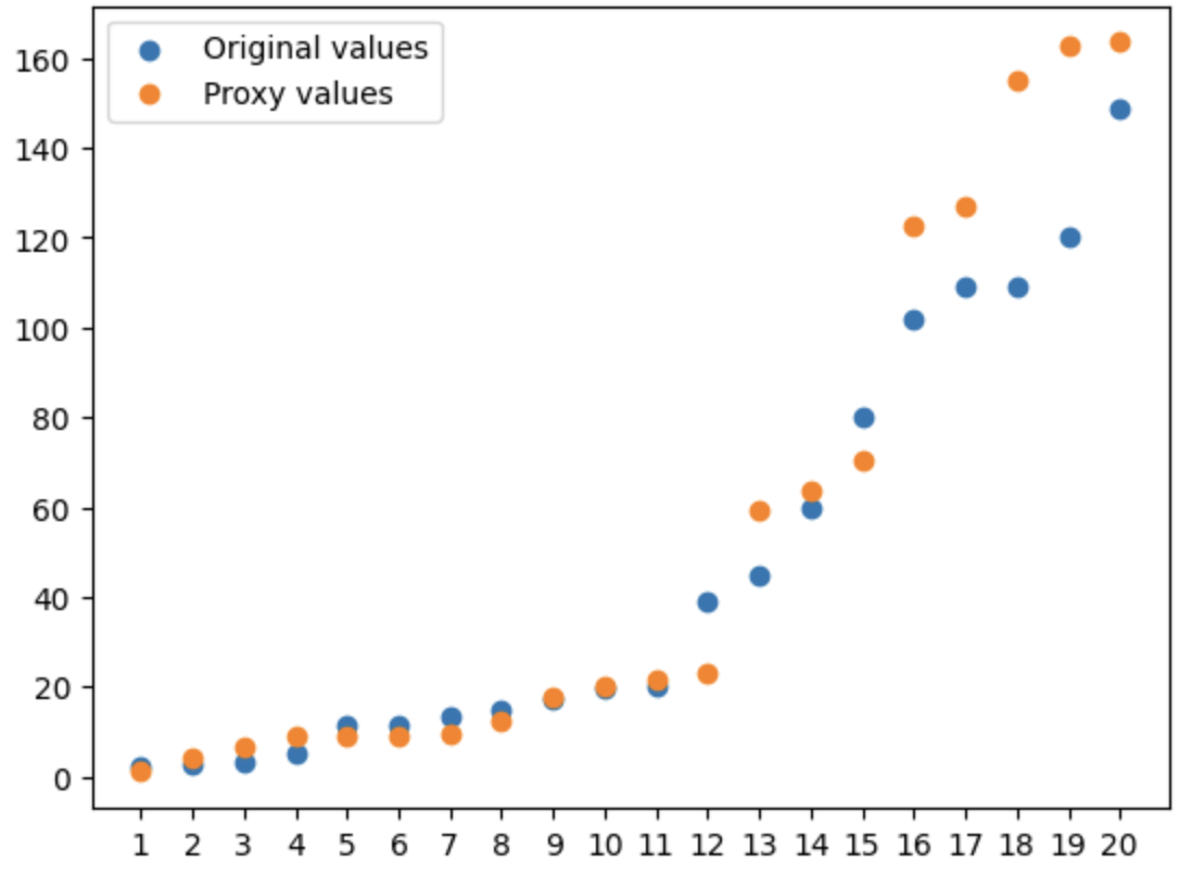
In a practical setting, we can’t assess the effectiveness of the Hard-Impute method by comparing the approximated values to the original ones, as the original values are missing. However, in the case of the US Arrests dataset, we have intentionally omitted 20 original values, enabling us to evaluate performance. The correlation coefficient between the approximated and original values is impressively high at 0.98, demonstrating the method’s efficiency. The scatter plot below visually supports our findings:
Proxied vs. Original values
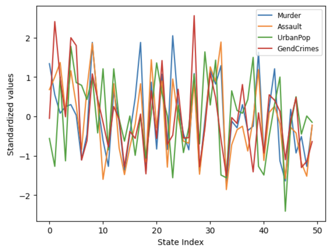
The Hard-Impute method has one significant limitation: it’s only suitable for numerical features. This means that if the dataset includes categorical or other non-numerical features, these need to be addressed separately. Additionally, it’s important to remember that the method’s efficiency is heavily influenced by the nature of the relationships between features. When features tend to vary in unison, their informational content can be more effectively encapsulated within the principal components, leading to more accurate reconstruction of missing values. For instance, in the US Arrests dataset, the logical co-occurrence of various types of crimes and the proportion of urban population contributes to the high efficiency of the Hard-Impute method. The line graph below illustrates how feature values generally trend together across most US states:
Co-movement of feature value s
Lastly, it’s crucial to address the significance of choosing the optimal number of principal components, denoted as M. With the US Arrests dataset, using M=1 yielded excellent results. However, the Hard-Impute method can accommodate any number of principal components. A strategy for determining the optimal M involves deliberately omitting extra values from the dataset, then applying the Hard-Impute method for all potential M values, and selecting the M that results in the highest average correlation between the approximated and original values.
Wrap-Up
Dear reader, we have now reached the end of this article. I hope you have found it insightful, and I trust you will agree that Hard-Impute is a valuable data preprocessing technique to include in your data science toolkit. For those interested in the Python code behind the algorithm, I encourage you to visit my git project. Additionally, I have published the method as a PYPI Python package, allowing for immediate installation and use of the algorithm.
Cheers!