Better Metric for ETF performance
If you are an ETF investor like myself, you probably inquiried about the performance of your favorite ETF before making a purchase. It is likely that your investment decision was to some extent influenced by the published rate of return — for example, QQQ at 9.44% per annum. Hopefully, besides the return, you also considered the fund’s risk often expressed in terms of beta or volatility. But what does the rate of return tell us? In particular, what do we mean when we say X% per annum?
How informative is the conventional rate of return?
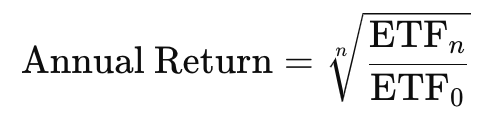
Annualized rate of return is a geometric mean over the individual annual returns, where the annual return rn is just a percentage change in ETF value within a particular year n:
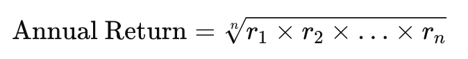
Annualized rate of return can also be expressed as the n-th root of the ETFs value increase over the holding period of n years:
Such rate of return is based on the assumption that an ETF was bought on a specific date (usually January 1st) and sold on the exact same date several years later. This scenario is quite unrealistic, given that an investor can buy or sell assets on any trading day of the year. With this in mind, I will demonstrate how the specific dates of purchase and sale can significantly influence the ETF’s annualized return rate. Let’s examine the performance of a very popular ETF - QQQ. The blue line represents a 5-year holding period from January 1, 2018 to January 1, 2023, while the red line shows a 5-year period from June 1, 2018, to June 1, 2023.”
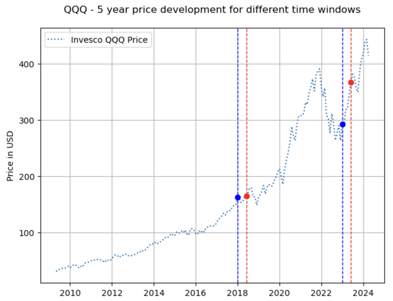
The blue and red time frames each span five years, overlapping over four and a half years. Despite this, the annualized rates of return, calculated using the second formula above, are 12.4% for the blue time window and 17.3% for the red time window. The choice of start and end date of the return calculation period have a huge impact on the rate of return. Essentially, if you are considering to purchase this ETF based on its annualized rate of return over the last five years, your decision could be heavily influenced by the most recent six-month period.
The start and end price have a huge impact on the conventional rate of return
In practice, an investor is likely to buy or sell her ETF on any given trading day of the year, and the holding period may not amount to a full n number of years. A typical investor often has limited knowledge about how long they will hold onto their investment - the holding period could range from months to decades, and this is usually not known in advance. Considering all of the points discussed, I have attempted to develop a more realistic metric for estimating ETF performance. This approach ensures that:
- The start and end dates of the return calculation period have the same importance as any other time point.
- Short-term and long-term holding periods are considered equally likely
To implement this, I am calculating n series of returns between data points that are m = n x 12 months apart, where n is the holding period expressed as the number of years (1, 2, 5, 7 and 10 years) - so 5 time series in total. Each series of returns is calculated as a rolling window, dividing the ETF price at time t+m by the ETF price at time t. The median of this series of returns represents the median n-year return for an ETF. For example, to obtain the median return over a 1-year holding period we would calculate a series of 12-month returns over a large window of consecutive months and find the median value. For a 5-year holding period, we would do the same but with 60-month returns.
The reader can see that the 1-year median return calculated in such a way is analogous to the annualized rate of return we described earlier.
Using this approach in our QQQ example, the blue and red time frames now yield median annual returns of 18.4% and 18.7%, respectively. These returns are now much more stable (compared to the previous 12.4% and 17.3%), and less dependent on the start and end date of the time frame chosen. This approach provides a clearer and more reliable comparison of the ETF’s performance against other competing ETFs.
Median returns over a roling price window is a more robust performance metric
One important aspect to remember is that the 1-year return rate is not meant to be compounded. For instance, a 5-year (median) return should not be calculated as (1.184%)5-1. Rather, to determine the 5-year return, we would apply the same procedure using m=60 interval.
After defining the implementation, the next step is to calculate this metric across a broad range of ETFs and various holding periods. The goal is to conduct a thorough comparison and obtain a clear indication of which ETFs have shown best historical performance. To achieve this, I processed a pool of approximately 21,000 ETF tickers available on the internet, from which around 5,500 were still active and had adequate and current data on Yahoo Finance.
Below is a series of ordered boxplots that summarize the performance of ETFs across holding periods of 1, 2, 5, 7, and 10 years. The plots on the left display the highest performance in terms of median return. The legend includes a description for each ETF, as available from the Yahoo Finance API, as well as a cumulative median return over the holding period (for example, the SOXX return of 9.8 for a 10-year holding period, means that the median return for this ETF over a 10 year period is $9.8 for every 1$ invested)
ETF performance report - output from the ETF_compare tool
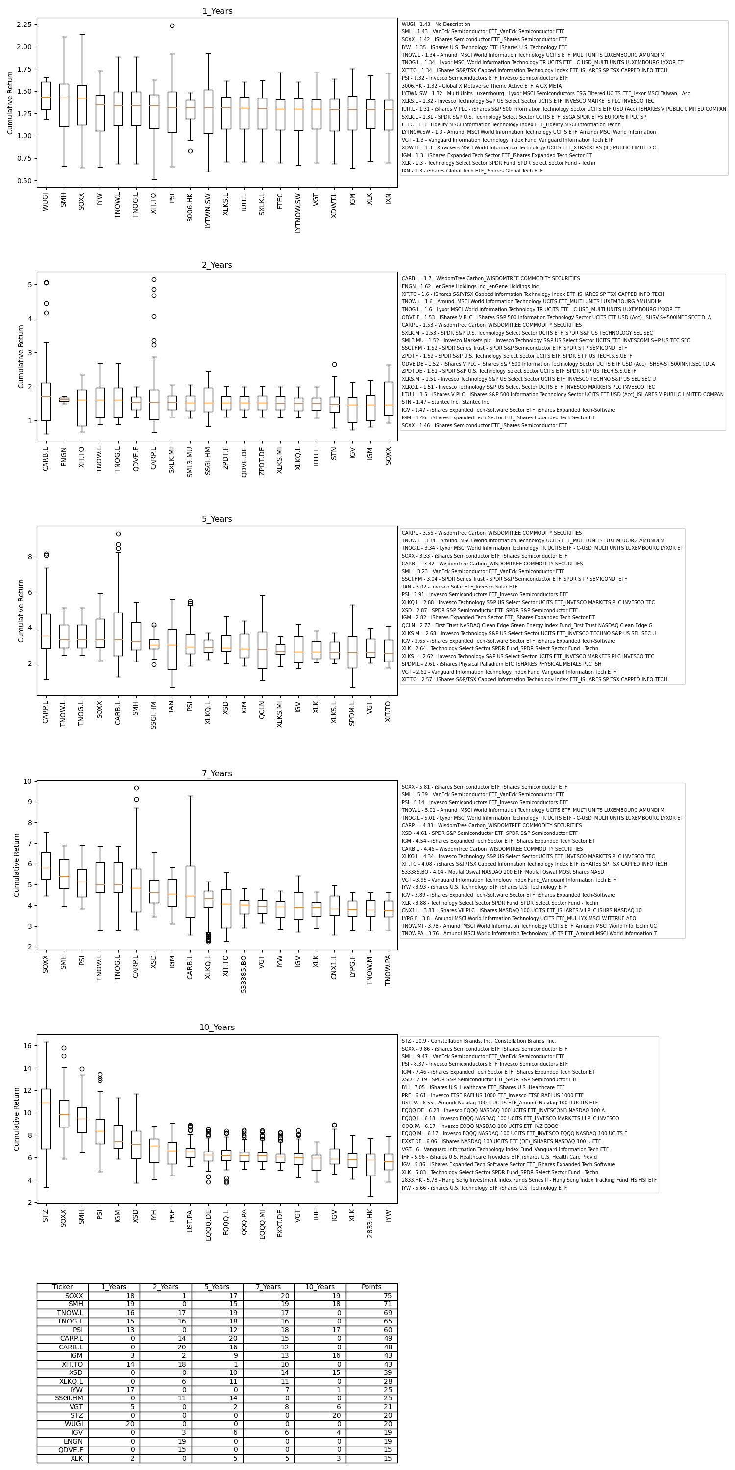
Unsurprisingly, many of the top-performing ETFs belong to the technology and semiconductor industries. Several ETFs show consistent high median returns across various holding periods. The table at the bottom of the report provides a comprehensive summary of the boxplots — the higher the median return an ETF achieves within a holding period, the more points it is allocated. For instance, if there are 20 ETFs/boxplots within a holding period, the ETF with the highest median return would receive 20 points. The best-performing ETFs overall are those with the highest total points across all holding periods. However, caution is needed as ETFs exhibit different return distributions, evident in the varying shapes of their boxplots.
Semiconductors and Technology lead the pack
Based on the bottom table, SOXX and SMH yield the highest median returns overall. However, for the 2-year holding period, the SOXX is at the last position and SMH is not even present in the best perfoming group. This is because the ETF performance for the 2-year holding period is very competititive, and it takes a small price movement for the ETFs to change rank. This is visible in the figure - the boxplot form an almost horizontal line. The technology ETFs TNOW and TNOG are following close behind, but they lack sufficient data for the 10-year holding period. These two ETFs are relatively new, having been established around 2010, and thus do not yet possess the minimum data history of 15 years required for a comprehensive long-term analysis. Further details about data time window used for each holding period are in the Notes section below.
I also strongly encourage the reader to make their own list of ETFs they wish to compare (see how in the Notes below). That way the reader can focus her comparison to a particular set of ETFs or a particular industry.
With this, we have come to the end of the post. I’ve made an effort to keep it brief and to the point, and I hope you have found it helpful. Please note that the topic of risk, specifically ETF price volatility, was not covered here, yet it is crucial for providing sound investment advice. The main objective of this post was to highlight the limitations of using conventional rates of return as indicators of ETF performance and to propose an alternative metric.
Notes:
Notes about the implementation:
- Data points are collected monthly, based on ETF prices at the beginning of each month. While daily data collection could improve precision, it would also require significantly more resources.
- To facilitate accurate comparisons between ETFs, the timeframe for calculating median returns is set as the holding period plus an additional 5 years. For example, a 10-year holding period would involve data stretching back 15 years from the most recent month, while a 1-year holding period would use data from the past 6 years.
- An ETF must have complete data for the past 6 months to be considered for analysis.
- An ETF with a data gap larger than 5 months is excluded.
- Smaller data gaps of less than 5 months are linearly interpolated to fill in missing values.
- An ETF must have at least 20 data points to be considered in the analysis.
- By default the leveraged ETFs are not included, however the user can include them if desired.
Notes about the code:
- The project and instructions how to run can be found in my Git repo
- The code runs on top of the yfinance library.
- The ETF_Ticker.csv file is included with the code and serves as the initial data source for the implementation.
- Users can add new tickers to the ETF_Ticker.csv to expand the dataset, or they can build a new file with only the tickers they select.
- Users can include additional ETFs for comparison against the best performers, provided that the ticker symbols are listed in the ETF_Ticker.csv file.
- Some tickers display inconsistent data, such as unexplainable jumps in values, and have thus been excluded from consideration.
- The Yahoo Finance API might occasionally return corrupted data for a given ticker - it is important to perform a sanity check