How Banks Decide on Your Loan
[Default Probability Modeling]
If you’ve had the experience of applying for a bank loan, you’re probably familiar with the fact that it’s quite a challenging process. It usually begins with an overwhelming amount of paperwork – forms to fill, guarantees to provide, and numerous signatures. But have you ever wondered how banks sift through all this information to decide who gets a loan and who doesn’t?
Banks essentially grapple with a fundamental question: Is the applicant capable of repaying the loan punctually, including interest and principal? A positive answer leads to loan approval, while a negative one results in rejection. The decision-making process has evolved significantly over the years. No longer relying solely on human judgment, banks have been embracing advanced classification algorithms for more than a decade now to enhance this process.
The task at hand is a classic example of a binary classification problem, one that today’s machine learning (ML) algorithms handle with remarkable efficiency. In the rest of this blog post, I’ll delve into the intriguing details of how this process works.
To begin with, banks must collect and compile a substantial dataset to effectively train their classification models. Here is a good example of such training dataset:
| loan_id | default | account_amount_added_12_24m | account_days_in_dc_12_24m | account_days_in_rem_12_24m | account_days_in_term_12_24m | account_incoming_debt_vs_paid_0_24m | account_status | account_worst_status_0_3m | account_worst_status_12_24m | account_worst_status_3_6m | account_worst_status_6_12m | age | avg_payment_span_0_12m | avg_payment_span_0_3m | merchant_category | merchant_group | has_paid | max_paid_inv_0_12m | max_paid_inv_0_24m | name_in_email | num_active_div_by_paid_inv_0_12m | num_active_inv | num_arch_dc_0_12m | num_arch_dc_12_24m | num_arch_ok_0_12m | num_arch_ok_12_24m | num_arch_rem_0_12m | num_arch_written_off_0_12m | num_arch_written_off_12_24m | num_unpaid_bills | status_last_archived_0_24m | status_2nd_last_archived_0_24m | status_3rd_last_archived_0_24m | status_max_archived_0_6_months | status_max_archived_0_12_months | status_max_archived_0_24_months | recovery_debt | sum_capital_paid_account_0_12m | sum_capital_paid_account_12_24m | sum_paid_inv_0_12m | time_hours | worst_status_active_inv |
|---|---|---|---|---|---|---|---|---|---|---|---|---|---|---|---|---|---|---|---|---|---|---|---|---|---|---|---|---|---|---|---|---|---|---|---|---|---|---|---|---|---|---|
| 39161 | 0.00000 | 0 | 0.00000 | 0.00000 | 0.00000 | 0.00000 | 1.00000 | 1.00000 | NaN | 1.00000 | NaN | 20 | 12.69231 | 8.33333 | 15 | 7 | 1 | 31638.00000 | 31638.00000 | 7 | 0.15385 | 2 | 0 | 0 | 13 | 14 | 0 | 0.00000 | 0.00000 | 2 | 1 | 1 | 1 | 1 | 1 | 1 | 0 | 0 | 0 | 178839 | 9.65333 | 1.00000 |
| 5668 | 0.00000 | 0 | 0.00000 | 0.00000 | 0.00000 | NaN | 1.00000 | 1.00000 | 1.00000 | 1.00000 | 1.00000 | 50 | 25.83333 | 25.00000 | 4 | 4 | 1 | 13749.00000 | 13749.00000 | 1 | 0.00000 | 0 | 0 | 0 | 9 | 19 | 3 | 0.00000 | 0.00000 | 0 | 1 | 1 | 1 | 1 | 2 | 2 | 0 | 0 | 0 | 49014 | 13.18139 | NaN |
| 84760 | 0.00000 | 0 | 0.00000 | 0.00000 | 0.00000 | NaN | NaN | NaN | NaN | NaN | NaN | 22 | 20.00000 | 18.00000 | 22 | 4 | 1 | 29890.00000 | 29890.00000 | 5 | 0.07143 | 1 | 0 | 0 | 11 | 0 | 3 | 0.00000 | 0.00000 | 1 | 1 | 1 | 1 | 1 | 2 | 2 | 0 | 0 | 0 | 124839 | 11.56194 | 1.00000 |
| 224 | 0.00000 | 0 | NaN | NaN | NaN | NaN | NaN | NaN | NaN | NaN | NaN | 36 | 4.68750 | 4.88889 | 22 | 4 | 1 | 40040.00000 | 40040.00000 | 2 | 0.03125 | 1 | 0 | 0 | 31 | 21 | 0 | 0.00000 | 0.00000 | 1 | 1 | 1 | 1 | 1 | 1 | 1 | 0 | 0 | 0 | 324676 | 15.75111 | 1.00000 |
| 78571 | 0.00000 | 0 | 0.00000 | 0.00000 | 0.00000 | NaN | NaN | NaN | NaN | NaN | NaN | 25 | 13.00000 | 13.00000 | 25 | 3 | 1 | 7100.00000 | 7100.00000 | 1 | 0.00000 | 0 | 0 | 0 | 1 | 0 | 0 | 0.00000 | 0.00000 | 0 | 1 | 0 | 0 | 1 | 1 | 1 | 0 | 0 | 0 | 7100 | 12.69861 | NaN |
| 4705 | 0.00000 | 0 | 0.00000 | 0.00000 | 0.00000 | NaN | NaN | NaN | NaN | NaN | NaN | 18 | NaN | NaN | 15 | 7 | 0 | 0.00000 | 0.00000 | 5 | NaN | 0 | 0 | 0 | 0 | 0 | 0 | NaN | NaN | 0 | 0 | 0 | 0 | 0 | 0 | 0 | 0 | 0 | 0 | 0 | 18.32833 | NaN |
| 16396 | 0.00000 | 0 | 0.00000 | 142.00000 | 0.00000 | 0.00000 | 1.00000 | 2.00000 | 2.00000 | 1.00000 | 3.00000 | 49 | 3.00000 | 3.00000 | 10 | 11 | 1 | 2373.00000 | 2373.00000 | 5 | 0.00000 | 0 | 0 | 0 | 1 | 0 | 0 | 0.00000 | 0.00000 | 0 | 1 | 0 | 0 | 1 | 1 | 1 | 0 | 18760 | 8337 | 2373 | 10.24444 | NaN |
| 34357 | 0.00000 | 57229 | 0.00000 | 0.00000 | 0.00000 | 0.23224 | 1.00000 | 1.00000 | 1.00000 | 1.00000 | 1.00000 | 34 | 26.93023 | 25.86667 | 22 | 4 | 1 | 8655.00000 | 9645.00000 | 0 | 0.08333 | 20 | 0 | 0 | 215 | 257 | 0 | 0.00000 | 0.00000 | 37 | 1 | 1 | 1 | 1 | 1 | 1 | 0 | 42206 | 35336 | 457257 | 12.19278 | 1.00000 |
| 19701 | 0.00000 | 148922 | 0.00000 | 47.00000 | 0.00000 | 0.96906 | 1.00000 | 2.00000 | 2.00000 | 2.00000 | 2.00000 | 40 | 33.72727 | 37.57143 | 22 | 4 | 1 | 6075.00000 | 9090.00000 | 6 | 0.81818 | 9 | 0 | 0 | 3 | 2 | 3 | 0.00000 | 0.00000 | 23 | 1 | 2 | 2 | 2 | 2 | 2 | 0 | 104643 | 32381 | 24390 | 21.41111 | 1.00000 |
| 83080 | 0.00000 | 0 | 0.00000 | 0.00000 | 0.00000 | NaN | NaN | NaN | NaN | NaN | NaN | 47 | 21.00000 | 21.25000 | 22 | 4 | 1 | 36985.00000 | 36985.00000 | 6 | 0.00000 | 0 | 0 | 0 | 5 | 10 | 0 | 0.00000 | 0.00000 | 0 | 1 | 1 | 1 | 1 | 1 | 1 | 0 | 0 | 0 | 78620 | 13.34083 | NaN |
The table presented above showcases an actual dataset from a fintech firm that operates as a consumer bank. For every loan given out, the bank collects information about account balances, previous loan records, financial background and demographic data of the applicant, at the time of application. The dataset in question is extensive, but not all the information it contains may be relevant. It’s a commonly accepted best practice to remove features that fail to provide extra value in the decision-making process. A time-tested method for identifying these redundant features involves calculating a correlation matrix for all features. By examining this matrix, one can easily spot features that exhibit a high correlation coefficient, indicating their potential redundancy.
Correlation matrix of the Dataset features
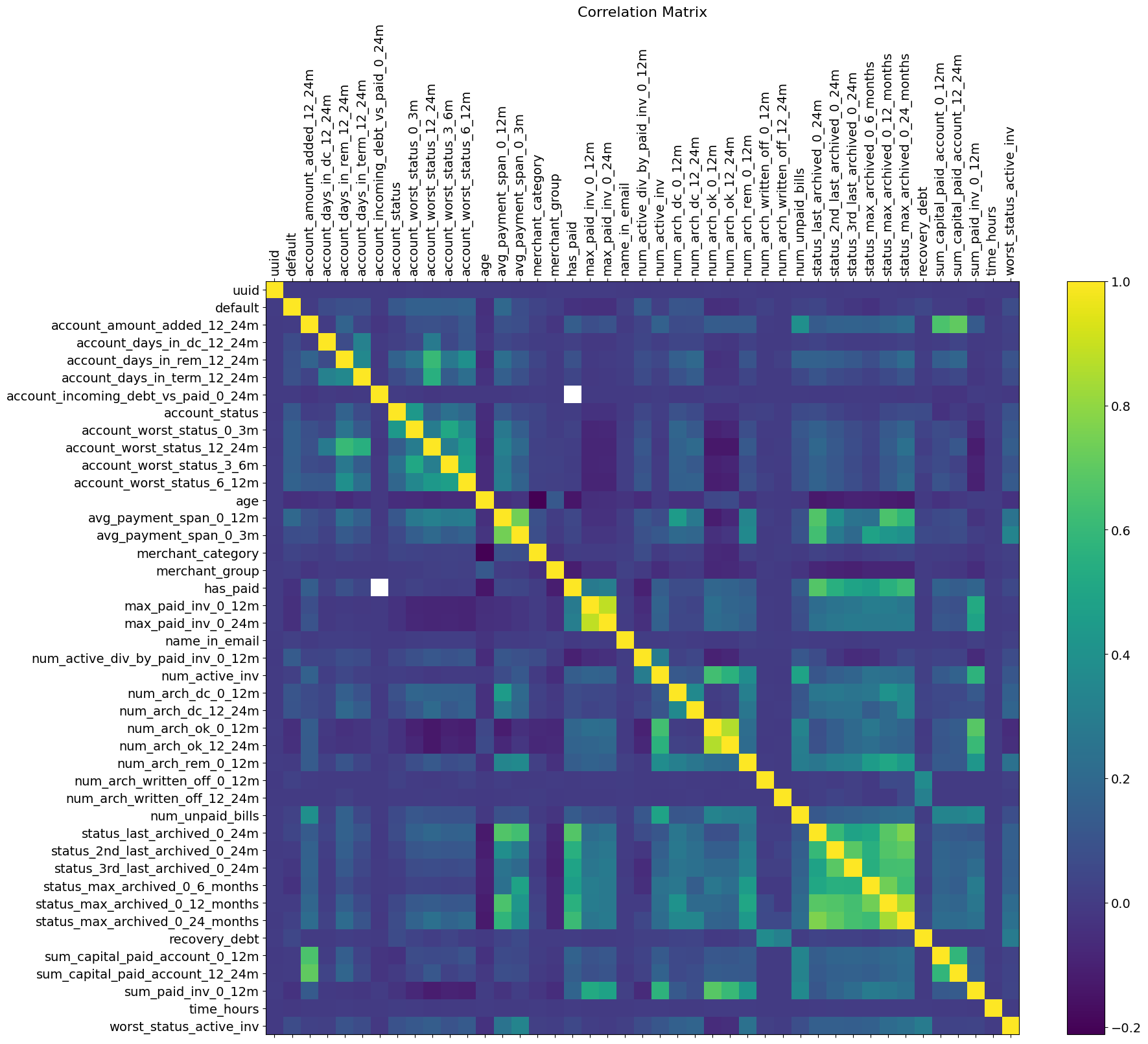
A critical information of this dataset is the “default” column, where each entry is either 0 or 1, indicating whether a customer has defaulted on their loan. This information is crucial for training the algorithm, and data records lacking this information can not be processed by the model. Another notable characteristic of this dataset is its sparsity, due to the frequent occurrence of missing values in loan applications. Prior to feeding this dataset to a classification model, it must undergo a specific encoding process. This process aims to effectively manage missing values and categorical features while simultaneously minimizing the loss of information. The financial sector commonly employs Weight-of-Evidence encoding due to its effectiveness in handling these challenges.
Weight-of-Evidence-Encoding
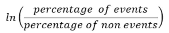
Weight of Evidence (WoE) encoding is a statistical method utilized in data preprocessing, particularly in machine learning for credit scoring and risk assessment. The technique focuses on converting categorical variables into a continuous scale. It does this by calculating the logarithm of odds associated with the target variable. Specifically, the WoE for each category is derived by taking the natural logarithm of the ratio of the proportion of positive outcomes to that of negative outcomes within that category. Such a transformation is key in highlighting the predictive strength of a categorical variable in relation to the target variable. This enables algorithms to more effectively process and learn from the data.
Additionally, WoE encoding treats missing values as distinct categorical entities. This approach avoids the pitfalls of discarding or replacing missing values with substitute figures, thus preserving the information of the dataset. Primarily designed for categorical data, WoE can also be adapted for numerical features with excessive missing values. This is achieved by categorizing these numerical values into bins and then applying WoE encoding. Below is an example of how an arbitrary categorical feature can be encoded with WOE. The number of events and non-events correspond to the count of binary values in the response variable (in our example the “default” column).
Example of Weight-of-Evidence encoding
| Feature-X(values) | Number of events | Number of non-events | Percentage events | Percentage non-events | WOE | IV |
|---|---|---|---|---|---|---|
| A | 90 | 2400 | 90/490=0.184 | 2400/9510=0.25 | Ln(0.184/0.25)=-0.3065 | 0.02 |
| B | 130 | 1300 | 130/490=0.265 | 1300/9510=0.137 | Ln(0.265/0.137)=0.659 | 0.175 |
| C | 80 | 3500 | 80/490=0.16 | 3500/9510=0.37 | Ln(0.16/0.37)=-0.838 | 0.176 |
| D | 100 | 1210 | 100/490=0.2 | 1210/9510=0.18 | Ln(0.2/0.18)=0.105 | 0.002 |
| E | 90 | 1100 | 90/490=0.184 | 1100/9510=0.12 | Ln(0.184/0.12)=-0.427 | 0.026 |
| Sum | 490 | 9510 | - | - | - | 0.399 |
The column WOE indicates a single feature’s predictive capability concerning its independent feature. When a category or bin within a feature displays a higher ratio of events relative to non-events, it yields a higher WoE value. High value of WoE suggests that the feature’s particular category or bin effectively discriminates between events and non-events. The formula to calculate the Weight-of-Evidence for any feature is:
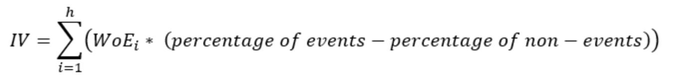
Lastly, it’s important to mention that a feature should typically meet a minimum threshold of information value to be included in the model otherwise it may simply add noise. The table’s final column displays the aggregated Information Value (IV), where we focus on the sum of IV across unique feature values. Generally, any feature with an aggregated IV below 0.02 is deemed non-significant. The aggregated IV statistic is calculated as follows:
After applying the WOE encoding, our dataset looks like this:
| loan_id | account_amount_added_12_24m_woe | account_days_in_dc_12_24m_woe | account_days_in_rem_12_24m_woe | account_days_in_term_12_24m_woe | account_incoming_debt_vs_paid_0_24m_woe | account_status_woe | account_worst_status_0_3m_woe | account_worst_status_12_24m_woe | account_worst_status_3_6m_woe | account_worst_status_6_12m_woe | age_woe | avg_payment_span_0_12m_woe | avg_payment_span_0_3m_woe | merchant_category_woe | merchant_group_woe | has_paid_woe | max_paid_inv_0_12m_woe | max_paid_inv_0_24m_woe | name_in_email_woe | num_active_div_by_paid_inv_0_12m_woe | num_active_inv_woe | num_arch_dc_0_12m_woe | num_arch_dc_12_24m_woe | num_arch_ok_0_12m_woe | num_arch_ok_12_24m_woe | num_arch_rem_0_12m_woe | num_arch_written_off_0_12m_woe | num_arch_written_off_12_24m_woe | num_unpaid_bills_woe | status_last_archived_0_24m_woe | status_2nd_last_archived_0_24m_woe | status_3rd_last_archived_0_24m_woe | status_max_archived_0_6_months_woe | status_max_archived_0_12_months_woe | status_max_archived_0_24_months_woe | recovery_debt_woe | sum_capital_paid_account_0_12m_woe | sum_capital_paid_account_12_24m_woe | sum_paid_inv_0_12m_woe | time_hours_woe | worst_status_active_inv_woe |
|---|---|---|---|---|---|---|---|---|---|---|---|---|---|---|---|---|---|---|---|---|---|---|---|---|---|---|---|---|---|---|---|---|---|---|---|---|---|---|---|---|---|
| 39161 | -0.20919 | -0.93784 | -0.86552 | -0.92614 | 0.14921 | -0.19706 | -0.06701 | -0.08080 | 0.02000 | 0.02000 | 1.11861 | 0.87745 | 1.90707 | 2.13021 | 1.57060 | -0.85294 | 1.90707 | 2.13021 | 0.47199 | 2.13021 | 1.43707 | -0.37531 | -0.39551 | 1.31928 | 1.57060 | -0.18479 | -0.81423 | -0.81423 | 0.87745 | -0.70300 | -0.64237 | -0.59437 | -0.45378 | -0.45378 | -0.24469 | -0.39551 | -0.17237 | -0.22116 | 0.00000 | 1.43707 | 0.25841 |
| 5668 | -0.20919 | -0.93784 | -0.86552 | -0.92614 | 0.06652 | -0.19706 | -0.06701 | 0.42547 | 0.02000 | 0.11531 | 1.57060 | 1.57060 | 2.41790 | 1.21392 | -0.37531 | -0.85294 | 0.47199 | 0.29763 | 0.62614 | -0.57784 | -0.09441 | -0.37531 | -0.39551 | -0.18479 | 1.57060 | 1.57060 | -0.81423 | -0.81423 | 0.11531 | -0.70300 | -0.64237 | -0.59437 | -0.45378 | 0.52078 | 0.05077 | -0.39551 | -0.17237 | -0.22116 | 1.57060 | 1.57060 | -0.09441 |
| 84760 | -0.20919 | -0.93784 | -0.86552 | -0.92614 | 0.06652 | 0.11531 | 0.11531 | -0.08080 | 0.08252 | 0.02000 | 1.43707 | 0.68329 | 1.43707 | -0.17237 | -0.37531 | -0.85294 | 2.13021 | 1.90707 | 0.42547 | -0.57784 | 0.95156 | -0.37531 | -0.39551 | 1.31928 | -0.23300 | 1.57060 | -0.81423 | -0.81423 | 0.80846 | -0.70300 | -0.64237 | -0.59437 | -0.45378 | 0.52078 | 0.05077 | -0.39551 | -0.17237 | -0.22116 | 1.90707 | 1.57060 | 0.25841 |
| 224 | -0.20919 | 1.50161 | 1.50161 | 1.50161 | 0.06652 | 0.11531 | 0.11531 | -0.08080 | 0.08252 | 0.02000 | 1.57060 | 1.72475 | 1.90707 | -0.17237 | -0.37531 | -0.85294 | 2.41790 | 2.41790 | 1.72475 | -0.57784 | 0.95156 | -0.37531 | -0.39551 | 1.43707 | 1.57060 | -0.18479 | -0.81423 | -0.81423 | 0.80846 | -0.70300 | -0.64237 | -0.59437 | -0.45378 | -0.45378 | -0.24469 | -0.39551 | -0.17237 | -0.22116 | 0.00000 | 1.43707 | 0.25841 |
| 78571 | -0.20919 | -0.93784 | -0.86552 | -0.92614 | 0.06652 | 0.11531 | 0.11531 | -0.08080 | 0.08252 | 0.02000 | 2.13021 | 0.74392 | 1.43707 | 2.41790 | 2.13021 | -0.85294 | 0.09878 | 0.27783 | 0.62614 | -0.57784 | -0.09441 | -0.37531 | -0.39551 | -0.18479 | -0.23300 | -0.18479 | -0.81423 | -0.81423 | 0.11531 | -0.70300 | 0.77567 | 0.65431 | -0.45378 | -0.45378 | -0.24469 | -0.39551 | -0.17237 | -0.22116 | 0.14921 | 1.31928 | -0.09441 |
| 4705 | -0.20919 | -0.93784 | -0.86552 | -0.92614 | 0.06652 | 0.11531 | 0.11531 | -0.08080 | 0.08252 | 0.02000 | 1.11861 | 0.91382 | 0.31784 | 2.13021 | 1.57060 | 1.11861 | 0.09878 | 0.27783 | 0.42547 | 0.91382 | -0.09441 | -0.37531 | -0.39551 | -0.18479 | -0.23300 | -0.18479 | 0.99078 | 0.99078 | 0.11531 | 0.99078 | 0.77567 | 0.65431 | 0.52078 | 0.91382 | 0.99078 | -0.39551 | -0.17237 | -0.22116 | 0.14921 | 1.43707 | -0.09441 |
| 16396 | -0.20919 | -0.93784 | 0.00000 | -0.92614 | 0.14921 | -0.19706 | 1.72475 | 1.72475 | 0.02000 | 0.00000 | 1.57060 | 1.72475 | 1.72475 | 1.72475 | 1.03160 | -0.85294 | 0.09878 | 0.27783 | 0.42547 | -0.57784 | -0.09441 | -0.37531 | -0.39551 | -0.18479 | -0.23300 | -0.18479 | -0.81423 | -0.81423 | 0.11531 | -0.70300 | 0.77567 | 0.65431 | -0.45378 | -0.45378 | -0.24469 | -0.39551 | 1.57060 | 2.41790 | 0.14921 | 1.43707 | -0.09441 |
| 34357 | 0.00000 | -0.93784 | -0.86552 | -0.92614 | 0.14921 | -0.19706 | -0.06701 | 0.42547 | 0.02000 | 0.11531 | 1.57060 | 1.57060 | 2.41790 | -0.17237 | -0.37531 | -0.85294 | 0.47199 | 0.29763 | 1.21392 | -0.57784 | 0.00000 | -0.37531 | -0.39551 | 0.00000 | 0.00000 | -0.18479 | -0.81423 | -0.81423 | 0.00000 | -0.70300 | -0.64237 | -0.59437 | -0.45378 | -0.45378 | -0.24469 | -0.39551 | 2.13021 | 2.41790 | 0.00000 | 1.31928 | 0.25841 |
| 19701 | 2.41790 | -0.93784 | 0.00000 | -0.92614 | 0.00000 | -0.19706 | 1.72475 | 1.72475 | 1.72475 | 1.90707 | 1.72475 | 2.41790 | 2.41790 | -0.17237 | -0.37531 | -0.85294 | 0.09878 | 0.29763 | 1.31928 | 0.00000 | 2.41790 | -0.37531 | -0.39551 | -0.18479 | -0.23300 | 1.57060 | -0.81423 | -0.81423 | 0.00000 | -0.70300 | 1.72475 | 1.72475 | 1.43707 | 0.52078 | 0.05077 | -0.39551 | 0.00000 | 0.00000 | 0.74392 | 1.90707 | 0.25841 |
| 83080 | -0.20919 | -0.93784 | -0.86552 | -0.92614 | 0.06652 | 0.11531 | 0.11531 | -0.08080 | 0.08252 | 0.02000 | 1.57060 | 1.72475 | 1.90707 | -0.17237 | -0.37531 | -0.85294 | 1.90707 | 2.13021 | 1.31928 | -0.57784 | -0.09441 | -0.37531 | -0.39551 | -0.18479 | -0.23300 | -0.18479 | -0.81423 | -0.81423 | 0.11531 | -0.70300 | -0.64237 | -0.59437 | -0.45378 | -0.45378 | -0.24469 | -0.39551 | -0.17237 | -0.22116 | 1.72475 | 1.57060 | -0.09441 |
The dataset is now prepared and set for the model to be executed. For brevity, I haven’t explained here the essential step of dividing the dataset into training, validation, and test subsets. However, it’s crucial for the reader to remember that the WOE encoding should be applied exclusively to the training subset. The validation and test datasets should be encoded by mapping their original values to the WOE-encoded values derived from the training set. Validation and test data are never encoded alongside the training data to prevent data leakage.
The Model
In binary classification tasks such as this, the finance sector frequently opts for the Logistic Regression (Logit) classifier model. This choice is standard in the industry for 3 reasons. First, the logit model produces a probability output, indicating the likelihood of an event being a “success” (in this context, it implies a loan default). This output is straightforward to understand and allows for the easy establishment of a customized threshold for success or failure, which can be different from the usual 0.5. Secondly, the Logit model provides us with a built-in feature importance for every independent variable of the model. And finally, the Logit model stands out as the most straightforward and easiest to understand classifier.
Recently, more advanced models have gained popularity among loan providers, offering an alternative to the traditional logit model. While the logit model’s simplicity is unmatched, certain complex models have been delivering consistently more accurate results, making them the preferred choice for some lenders. One such model is XGBoost, an efficient and scalable variant of the boosting family of models. As an ensemble learning method, XGBoost constructs multiple models (specifically decision trees) and amalgamates them for improved accuracy and robustness. The models are added in sequence during training, each addressing the errors of its predecessors until no further enhancements are possible. Similar to the Logit model, XGBoost predicts the probability of “success”. However, it’s more intricate to train due to the extensive calibration of numerous hyperparameters required throughout the training phase.
Hyperparameter tuning or calibration is a key aspect of this model. This process involves creating a grid encompassing all sensible values of the hyperparameters. For each unique combination of these hyperparameters, the model undergoes training, and the set of hyperparameters that produces the most optimal result (be it in terms of Accuracy, F1 Score, Recall, or any other metric chosen by the model developer) is identified and retained. The model trained with this set of hyperparameters is often referred to as the “champion model.” This model is then applied to test data, which in our context means predicting the likelihood of loan defaults for new loan applications. In the following, we will go through some of the common hyperparameters of the XGBoost model:
Example of a hyperparameter grid
param_grid = {
        'learning_rate': [0.01, 0.01],
        'max_depth': [8, 9, 10],
        'subsample': [0.8, 0.7, 0.6],
        'colsample_bytree': [0.9, 0.8],
        'scale_pos_weight': [70]
        'reg_alpha': [0.1, 0.5]
    }
learning_rate: determines the impact of each tree on the final outcome. A smaller learning rate requires more boosting rounds to achieve the same reduction in residual error as a larger learning rate. Common values are in the range of 0.01 to 0.3.
max_depth: defines the maximum depth of a tree. Deeper trees can model more complex patterns, but they are also more likely to overfit. The values in the grid (8, 9, 10) suggest moderately deep trees.
subsample: sets the fraction of the training data to be randomly sampled for each tree. Values below 1 make the algorithm more conservative and prevent overfitting but too small values might lead to underfitting.
colsample_bytree: The fraction of features to be randomly sampled for each tree. Values less than 1 help in making the model more robust by reducing overfitting and can be particularly useful for datasets with a large number of features.
scale_pos_weight: Used in imbalanced classification to scale the gradient for the minority class. A value of 70 suggests that the problem is quite imbalanced, and the model should increase the importance of the minority class by a factor of 70.
reg_alpha: The L1 regularization term on the weights (also known as alpha). Regularization helps to prevent overfitting by penalizing more complex models.
The full list of potential hyperparameters is extensive, and it is available here. To run this model efficiently it is important to understand well the mechanism of the model and the impact of its parameters.
After training the champion model, the next step is to test it on the validation dataset to evaluate its performance. If the results meet our expectations and criteria on the validation set, we can then move forward to deploy the model in a real-world setting. This means the model will be used to determine whether new customers are eligible for loan approval or not. This approach is reflective of how modern banking systems process loan approvals.
We’re now set to run our champion model on the WOE encoded validation data. It’s important to note that our model was trained using the fairly light parameter grid outlined earlier. Training the XGBoost model with an extensive grid on a personal computer can be an extremely time-intensive task. Consequently, our parameter tuning and model results could likely be improved conditional we had access to greater computational resources. Our model yields the following results on the validation dataset:
AUC-ROC: 0.8868571946417096
Recall: 0.7372262773722628
Precision: 0.08054226475279107
AUC-PR: 0.12131912757189459
Confusion Matrix:
[[7707 1153]
 [  36  101]]
This dataset exhibits a significant imbalance, making the accurate identification of defaults more critical than the occasional mislabeling of non-defaults. In this context, the relatively high recall metric is a positive aspect, as it indicates a good rate of correctly identifying actual defaults. However, the precision is notably low, suggesting that only a small fraction of loans predicted to default actually do so. This could mean the model is overly cautious, potentially rejecting financialy healthy customers, which is not beneficial for the business. Another interesting observation is the stark contrast between the AUC-ROC and AUC-PR metrics, which again underlines how important it is to consider the use of AUC-PR instead of the AUC-ROC metrix when faced with an imbalanced dataset.
Executing the champion model on a batch of fresh loan applications would produce the following probabilities of default:
| loan_id | default_probability |
|---|---|
| 349 | 0.23701356 |
| 44 | 0.19725785 |
| 8411 | 0.2826372 |
| 693 | 0.4592986 |
| 676 | 0.6802527 |
| 70 | 0.33273283 |
| 598 | 0.2290507 |
| 66790 | 0.28260818 |
| 1470 | 0.47338352 |
| 79385 | 0.27572608 |
| 2894 | 0.40206018 |
As anticipated, the default probabilities vary between 0 and 1, with just a single loan application showing a default probability above 0.5. In a practical scenario, this would mean that the loan with ID 676 is likely to be denied approval.
Dear reader, we have reached the end of this post. I hope you’ve found it enlightening and that it has given you a deeper understanding of the mechanics behind loan applications. Instead of a bank official reviewing your documents, it’s quite probable that a sophisticated algorithm in the bank’s infrastructure is making the decision about your loan approval. For those interested in delving deeper into this subject, I encourage you to visit my git project. There you can explore the entire dataset, examine the code implementation in detail, or even download the model as a Docker application.
Thank you for reading and I wish you a 0% default probability!